
Industry
The industrial sector in US-REGEN is modeled in detail for some sectors and technologies, including iron & steel, cement, and steam demand from boilers across all manufacturing sectors, while other industrial energy use is modeled with a more aggregate representation. Note that non-manufacturing energy use is modeled as part of non-road vehicles and equipment.
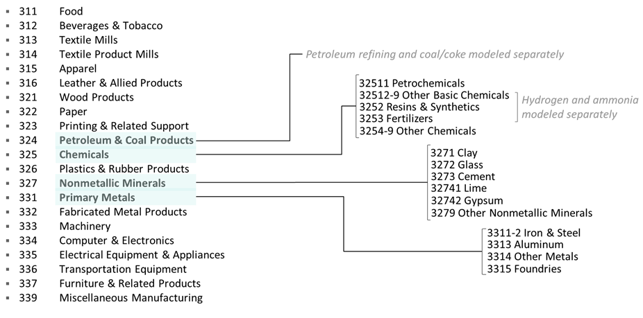
The allocation of base year energy consumption across sectors and end-uses on a regional basis is the result of a calibration exercise bringing together information from SEDS, the Manufacturing Energy Consumption Survey (MECS) conducted by the EIA, the Advanced Manufacturing Office from DOE, and published NEMS results in AEO. The sectoral definitions mostly follow the categorization used by AEO and NEMS, as summarized in Figure 1.
Boilers
This segment includes cost and performance of existing boiler stock across the industrial sectors, as well as new boilers that may be required to meet future demand under different scenarios.
Existing boilers can use a range of fuels including diesel, residual fuel oil, other petroleum fuels, pipeline gas, coal, electricity, or biomass. Boiler efficiencies vary by fuel type, with biomass boilers being the least efficient at around 75%, gas and petroleum fuels between 80-85%, and electric boilers up to 99%, estimated based on data from MECS. Potential new boiler types were assumed to have efficiencies that vary by fuel type and are presented in Table 1. Boilers are assumed to have a model life of 30 years in most cases, except for electric and heat pump boilers which are assumed to stay online for 15 years after installation.
| New Boiler Technology | Efficiency |
|---|---|
| Electric | 99.0% |
| Coal | 90.3% |
| Gas | 85.7% |
| Liquid Fuel | 89.0% |
| Hydrogen | 85.7% |
| Biomass | 75.0% |
| Heat Pumps > 50C | 280% |
| Heat Pumps < 50C | 600% |
Boilers can produce steam at different temperatures—for this modeling, four discrete temperature bands are selected—below 50C, 50-100C, 100-250C and >250C. While the efficiencies of these boilers are generally assumed to depend on their type, they are not assumed to vary by temperature class. The exception is for heat pumps where the COP for the <50C temperature class heat pump boilers is higher than the 50-100C class. Another distinction is that not all boiler types can meet all temperature classes. For example, heat pump boilers can only supply steam up to 100C, most other boilers can go up to 250C, while only coal, gas, and hydrogen boilers can supply steam up to 500C.
Assumed cost data for new boilers are summarized by technology type in Table 2.[1]
| New Boiler Technology | Capital Cost ($/kWth) | FOM ($/kW-yr) |
|---|---|---|
| Electric | 189 | 1.2 |
| Coal | 315 | 16 |
| Gas | 269 | 13 |
| Liquid Fuel | 234 | 12 |
| Hydrogen | 309 | 15 |
| Biomass | 282 | 14 |
| Heat Pumps | 888 | 27 |
All values are shown in 2015 USD terms.
Existing boiler stock, distinguished by temperature class and industrial sector, is estimated based on data in MECS and NREL's "Manufacturing Thermal Energy Use in 2014" report. All existing boiler stock is assumed to stay online for modeled lifetimes past the base year, after which replacement is required. Policy or other factors may drive the early retirement and replacement of some of these existing units. Both existing and new boilers are limited to annual capacity factor thresholds that vary between 25% and 90% depending on the industrial sector they are used in and are based on available historic data. Steam demand is assumed to scale with industrial service demand in future years, which are projected based on national trends in the AEO for each industrial sector. Additionally, the share of boiler demand by temperature class in each industrial sector is assumed to remain the same in future years. Additional demand arises from steam requirements for industrial CCS pathways in the cement and iron & steel sectors as determined endogenously.
Cement
REGEN estimates the energy required to produce cement in the U.S. under different future scenarios. Energy demand across all the end uses (e.g. process heat, HVAC, machine drives) in the cement industry is aggregated by fuel type (e.g. gas, coal, electricity), based on data from USGS. Future demand for cement is projected based on national trends in the AEO, and associated fuel demands are assumed to grow proportionally, with no future efficiency improvements. Process emissions from calcination are represented as 0.55 tonne CO2 per tonne cement produced based on data from historic data from DOE.
Existing plant capacity is estimated from USGS data that reports annual production and percent utilization by region. Existing cement plants are assumed to stay online until 2050; however, policy or other drivers may drive earlier retirement and replacement. To meet demand that is unmet by existing plants, new plants without or with post-combustion carbon capture can be added, and technoeconomic data for these new plants are based on inputs from IEA. In general, plants with carbon capture are assumed to capture 85% of the process emissions from calcination, and have higher capital and operating costs, as well as higher energy requirements. The capture pathway requires additional steam for CO2 stripping and electricity for CO2 compression, the costs and production of which are endogenously captured within REGEN. Cement sector decarbonization can also occur through fuel switching to low-carbon alternatives.
Iron & Steel
The iron & steel sector within REGEN is modeled via several pathways that produce primary and secondary steel (Figure 2).
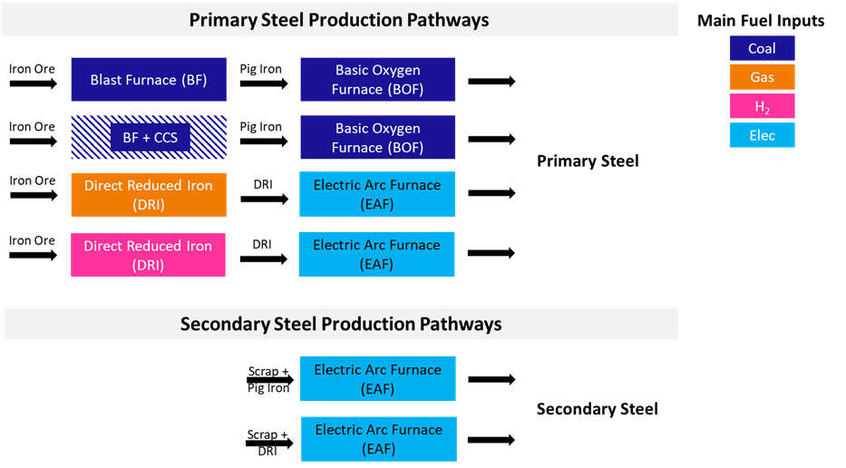
The model represents the two steps in the production of steel—the transformation of raw iron to the intermediate products of pig iron or direct reduced iron (DRI), and then the conversion of these commodities to steel (see Figure 2). Pig iron is produced using a blast furnace with coal as a primary fuel input (Figure 2, row 1). Besides this pathway, REGEN also includes an alternate technology pathway where carbon can be captured at the blast furnace (Figure 2, row 2), with a 74% capture rate on embedded emissions of 0.23 tonnes of CO2 per tonne of iron. An alternative is to use either natural gas or hydrogen to make DRI (Figure 2, rows 3 and 4). The remaining commodity that can be used to produce steel is scrap or recycled steel, which is primarily used to produce secondary steel.
Using different mixes of these commodities, primary and secondary steel can be produced using either an electric arc furnace or a basic oxygen furnace. The basic oxygen furnace is the traditional way of producing primary steel from pig iron and a small amount of scrap metal (Figure 2, rows 1 and 2). Steel plants generally include both a blast furnace and basic oxygen furnace. The traditional way to produce secondary steel is using an electric arc furnace with scrap and a little pig iron as inputs (Figure 2, row 5). Alternatively, scrap can be mixed with DRI that has been produced using either natural gas or hydrogen to produce secondary steel (Figure 2, row 6). In addition, primary steel can be produced using DRI and scrap using an electric arc furnace (Figure 2, rows 3 and 4).
Future steel demand is projected from national trends in the AEO and assumes that 30% of the demand is for primary steel, similar to historic shares of primary steel production in the U.S. Regional demand for primary and secondary steel is assumed to be consistent with regional shares in 2015 (as determined by data from USGS and USGHGRP). Secondary steel is assumed to use 95% scrap while primary uses 11-18% scrap.
Existing plant capacity is estimated from USGS and USGHGRP data on annual production of primary and secondary steel as well as regional shares and assumed utilization factors of 85% based on historic averages. Existing plants are assumed to stay online until 2050, however policy or other drivers may drive earlier retirement and replacement. Energy used for the existing pathways (blast furnace for pig iron, basic oxygen furnace for primary steel and electric arc furnace for secondary steel production) are estimated using data from AEO and are aggregated across end-uses by fuel type. Technoeconomic data for alternate pathways are determined based on available literature. Cost data for the alternate pathways are summarized in Table 3.
| Technology | Capital Cost ($/tpa) | FOM ($/tpa-yr) | VOM ($/tonne) |
|---|---|---|---|
| Blast furnace for pig iron production | 540 | 54 | 182 |
| Blast furnace for pig iron production with CCS | 700 | 58 | 182 |
| DRI production with natural gas | 479 | 54 | 149 |
| DRI production with H2 | 308 | 54 | 149 |
| Basic oxygen furnace for primary steel production | 278 | 0 | 128 |
| Electric arc furnace for primary steel production | 408 | 20 | 98 |
| Electric arc furnace for secondary steel production | 408 | 20 | 277 |
All values are shown in 2015 USD terms.
Other Manufacturing Sectors and Technologies
The remaining manufacturing sectors and technologies are modeled in a more stylized manner. Once the base year has been established, service demands for each end-use are projected based on national trends in the AEO for each industrial sector. Service demands by end-use within industrial sectors are projected to grow proportionally to sectoral output. That is, the model assumes that the relative shares of process heating and cooling versus machine drive and non-process services such as facility lighting and HVAC do not change over time, nor does the relative share of energy services in industrial output. While within-industry structural change may result from technical change, these trends are difficult to predict. However, the model does assume the energy per service unit declines over time, at different rates depending on the end-use (see Table 4). These rates are exogenously specified, but the model also includes the option to accelerate the rate of efficiency improvement (at an additional cost) in response to rising energy prices.
| Annual rate | |
|---|---|
| Process heating / cooling | 0.8% |
| Machine drive | 1.0% |
| Non-process industrial use | 0.8% |
The model formulation then evaluates trade-offs between supplying service demand across a stylized set of candidate technologies corresponding to alternative fuels (for example, electric, gas, hydrogen, biomass). The parameterization of these trade-offs is simpler than that described for buildings and transportation, but involves the same conceptual components: a relative coefficient of performance determining energy consumption and cost, and a non-energy cost component reflecting capital costs as well as productivity improvements or other service improvements. Table 5 summarizes assumptions for relative coefficient of performance, that is, relative fuel use per service unit, for industrial end-uses. Missing values indicate technology/end-use combinations. Non-energy costs are based on top-down assumptions rather than bottom-up assessments of the underlying technologies for these industrial sectors. In general, electric end-use technologies are assumed to have similar or in some cases lower capital and operating costs. As an example, Table 6 summarizes the relative capital costs of candidate technologies for process heating, indexed to the benchmark natural gas technology. The levelized capital cost of process heating equipment for the natural gas technology relative to energy consumption is assumed to be $61 per MMBtu of final energy consumption. These parameters are based on information in EPRI's Electrification Knowledge Base.
| Electric | Advanced Electric | Coal | Gas | Liquids | Bio | Hydrogen | |
|---|---|---|---|---|---|---|---|
| Process cool | 1.0 | ||||||
| Process heat | 1.0 | 1.5 | 1.0 | 1.0 | 1.0 | 1.0 | |
| Electrochemical process | 1.0 | ||||||
| Co-gen boiler | 1.0 | 1.0 | 1.0 | 1.0 | 1.0 | 1.0 | |
| Machine drive | 1.0 | 0.3 | |||||
| Industrial facilities HVAC | 1.3 | 2.0 | 1.0 | 1.0 | 1.0 | ||
| Industrial facilities lighting | 1.0 |
| 2020 | 2025 | 2030 | 2035 | 2040 | 2045 | 2050 | |
|---|---|---|---|---|---|---|---|
| Electric | 0.8 | 0.8 | 0.8 | 0.8 | 0.8 | 0.8 | 0.8 |
| Advanced Electric | 1.1 | 1.1 | 1.1 | 1.1 | 1.1 | 1.1 | 1.1 |
| Gas | 1.0 | 1.0 | 1.0 | 1.0 | 1.0 | 1.0 | 1.0 |
| Liquids | 1.1 | 1.1 | 1.1 | 1.1 | 1.1 | 1.1 | 1.1 |
| Hydrogen | 1.2 | 1.1 | 1.0 | 1.0 | 0.9 | 0.8 | 0.8 |
Han, et al. (2017). A Techno-Economic Assessment of Fuel Switching Options of Addressing Environmental Challenges of Coal-Fired Industrial Boilers, Energy Procedia, 142, 3083-3087; TNO (2018). Technology Factsheet for Electric Industrial Boiler. ↩︎